Machine learning basics
After my last post on data analysis, I will now briefly describe how to achieve a good score for the Titanic survival classification, the house prices regression, and the NLP twitter disaster problems in Kaggle. The caret library in R makes it easy to test different machine learning algorithms.
Machine learning
Machine learning algorithms are able to learn from past data how to make predictions on new data. The most common types of ML algorithms are supervised or unsupervised.
Supervised algorithms are used to solve classification (predict a class) and regression (predict continuous variable) problems. Training data contains labels and common metrics to evaluate models are accuracy, precision and recall for classification, or root mean square error (RMSE) and R-squared (R2) for regression. Prediction of time series can be made using other type of statistical models, like ARIMA and prophet.
Unsupervised algorithms usually consist on dimensionality reduction (PCA, SVD, t-sne), clustering (hierarchical, k-means, DBSCAN), anomaly detection and a few others. These do not require training data, and there are different techniques to evaluate each algorithm.
Classification
The Titanic problem is a binary classification problem that consists on predicting the passengers who survived the disaster. Let’s take a look at the data.
1 | > glimpse(titanic_train) |
Feature engineering can be more important than the machine learning algorithms applied. Some features like Cabin contain too many missing values and should be dropped. Other features may added, like the Title (Mr, Ms) from the name, or the Fsize (family size) taking into account the SibSp (siblings/spouses), Parch (parents/children) and Ticket (number of duplicate tickets). Any missing values in the observations must be imputed.
As a baseline, since most people died, a naive algorithm could predict that all people died and would achieve 62% accuracy on the train set. A smarter baseline model would predict that all men died and women survived, which would result in 79% accuracy. A machine learning algorithm should recognize patterns in the data and have better accuracy. Cross-validation (CV) is useful to prevent models from overfitting (achieving high train accuracy but low test accuracy).
I’ve tried logistic regression, random forest, gradient boosting, however the algorithm that achieved best results in Kaggle was a simple tree classifier with 83% CV accuracy and 80% accuracy in the test set. The smart baseline would result in 77% test accuracy, so a small improvement was made.
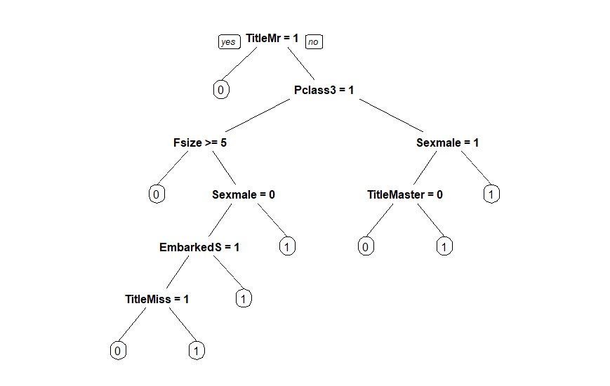
With this decision tree, the Title, Pclass, Fsize, Sex and Embarked are the features used to decide the fate of a passenger. A simple visualization of the train data shows hints on why this tree was made.
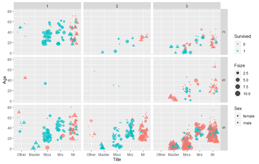
The tree is very interpretable. It captures that on Pclass 3, big families die, as well as Misses who embarked on S. For Pclass 1 and 2 it predicts that children and women live.
Regression
For this problem the predicted variable, Price, is skewed to the right, so a log transformation is helpful to make the distribution more normal and improve the predictions. The train dataset contains 1460 observations and 81 variables, most of which are useless.
A lot of feature engineering was done to improve the predictions. A few variables have missing values but can be imputed with related variables. Right skewed variables should be transformed using a log function. Encoding a few categorical values as ordinals and removing outliers also improves results. A correlation matrix is helpful to select the most important features for models that are sensitive to multicollinearity, like linear regression.
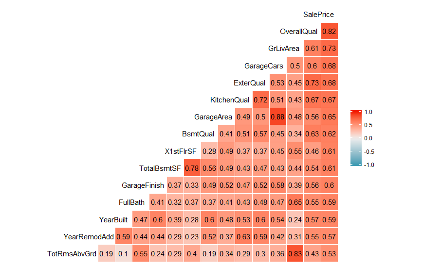
Lasso regression achieved 0.11183 CV RMSE and 0.11911 test RMSE. Elasticnet was close behind, while ridge/linear regression and gradient boosting were worst but still an improvement over a mean baseline.
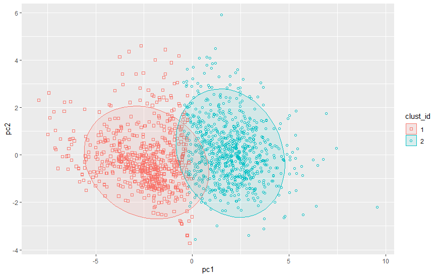
To improve results I used k-means clustering to create 2 clusters and train a lasso model for each cluster. With this approach, the cluster for each test observation had to be predicted. Performance improved to 0.11897 RMSE. I have seen this cluster and then predict with linear models (not really needed for tree based models) approach in the EDX MOOC called The Analytics Edge, which I do recommend as it was very practical, easy to follow, covered many topics and included many examples and exercises.
With a weighted combination of all models, a final 0.11765 RMSE was reached, which at the time was enough to be in the top 20%. To further improve results more feature engineering and hyperparameter tuning would be required.
NLP
For this natural language problem I have used the R quanteda library, which contains many helpful methods for text mining. Besides statistical analysis, NLP techniques like stemming and lemmatization can be used. One of the most helpful ways to compare the most used words in tweets that have been labeled as disaster or not is to plot a wordcloud.
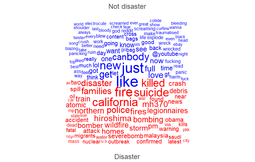
The data was not clean, there were duplicate tweets with different labels, so the best approach is to use the mode to select the right label. To try a ML algorithm, text must be transformed to tabular data, where each row is a tweet, or document, and each column is a word, or feature. For the feature value I had best results with the word count, but binary encoding or tf-idf are also valid choices. Additional features like number of URLs and # also improved model performance.
Since the resulting matrix is sparse and has many dimensions, it is helpful to remove words/columns that rarely appear. Naive bayes and Linear SVM algorithms are often used for text classification because they are fast to train on high dimensional data and provide good results. For more demanding models to train faster, a dimensionality reduction algorithm (e.g.: LDA, LSA) is typically applied first. With SVM I was able to reach 83% CV accuracy and 80% test accuracy. Bigrams did not improve the model but ensembles probably could. Using a part of speech tagger and filtering word classes like nouns/verbs can help.
Unsupervised techniques to generate dense word embeddings like word2vec, based on neural networks, and GloVe, based on word co-occurrence, or even simpler PMI+SVD approaches are quite interesting. Words used in similar contexts will be closer in the vector space and documents are compared with cosine similarity by averaging the word vectors. Using these vectors, documents can be searched using approximate k-NN methods. Recently, other techniques/models have achieved good results in some tasks, such as BERT, which captures contextual embeddings, fastText, that learns vectors from character n-grams, doc2vec, GPT-2, and the list goes on.
Conclusion
I am satisfied with the results obtained and was able to learn more about machine learning. I did not explain everything and did not include any code on this post, feel free to check the code on github which contains more comments. R is fine for data analysis, but I would recommend Python if you want to deploy your ML workloads in production and if you want to use state of the art NLP models.